1 Installation

This workshop uses a data bundle. Download it and extract to a convenient location.

To explore the PostgreSQL/PostGIS database, and learn about writing spatial queries in SQL, we will need some software, either installed locally or available remotely on the cloud.

There are instructions below on how to access PostgreSQL for installation on Windows or MacOS. PostgreSQL for Windows and MacOS either include PostGIS or have an easy way to add it on.
There are instructions below on how to install PgAdmin. PgAdmin is a graphical database explorer and SQL editor which provides a "user facing" interface to the database engine that does all the world.

For always up-to-date directions on installing PostgreSQL, go to the PostgreSQL download page and select the operating system you are using.

1.1 PostgreSQL for Microsoft Windows

For a Windows install:

Go to the Windows PostgreSQL download page.
Select the latest version of PostgreSQL and save the installer to disk.
Run the installer and accept the defaults.
Find and run the "StackBuilder" program that was installed with the database.
Select the "Spatial Extensions" section and choose latest "PostGIS ..Bundle" option.
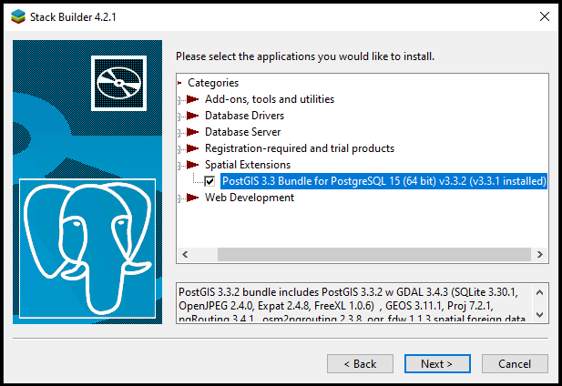
Accept the defaults and install.

1.2 PostgreSQL for Apple MacOS

For a MacOS install:

Go to the Postgres.app site, and download the latest release.
Open the disk image, and drag the Postgres icon into the Applications folder.
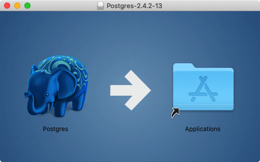
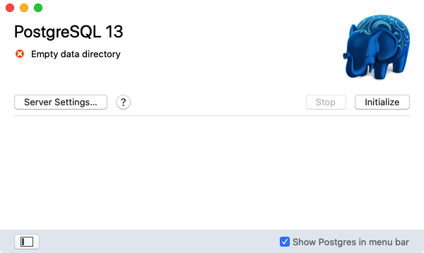
In the Applications folder, double-click the Postgres icon to start the server.
Click the Initialize button to create a new blank database instance.

{.inline, .border .inline, .border}
In the Applications folder, go to the Utilities folder and open Terminal.
Add the command-line utilities to your PATH for convenience.

sudo mkdir -p /etc/paths.d
echo /Applications/Postgres.app/Contents/Versions/latest/bin | sudo tee /etc/paths.d/postgresapp

1.3 PgAdmin for Windows and MacOS

PgAdmin is available for multiple platforms, at https://www.pgadmin.org/download/.

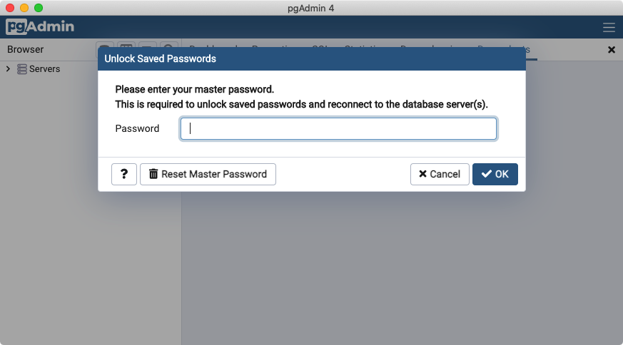
Download and install the latest version for your platform.
Start PgAdmin!

2 Creating a Spatial Database

2.1 PgAdmin

PostgreSQL has a number of administrative front-ends. The primary one is psql, a command-line tool for entering SQL queries. Another popular PostgreSQL front-end is the free and open source graphical tool pgAdmin. All queries done in pgAdmin can also be done on the command line with psql. pgAdmin also includes a geometry viewer you can use to spatial view PostGIS queries.

Find pgAdmin and start it up.
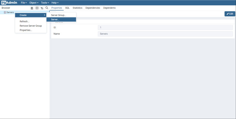
If this is the first time you have run pgAdmin, you probably don't have any servers configured. Right click the Servers item in the Browser panel.

We'll name our server PostGIS. In the Connection tab, enter the Host name/address. If you're working with a local PostgreSQL install, you'll be able to use localhost. If you're using a cloud service, you should be able to retrieve the host name from your account.

Leave Port set at 5432, and both Maintenance database and Username as postgres. The Password should be what you specified with a local install or with your cloud service.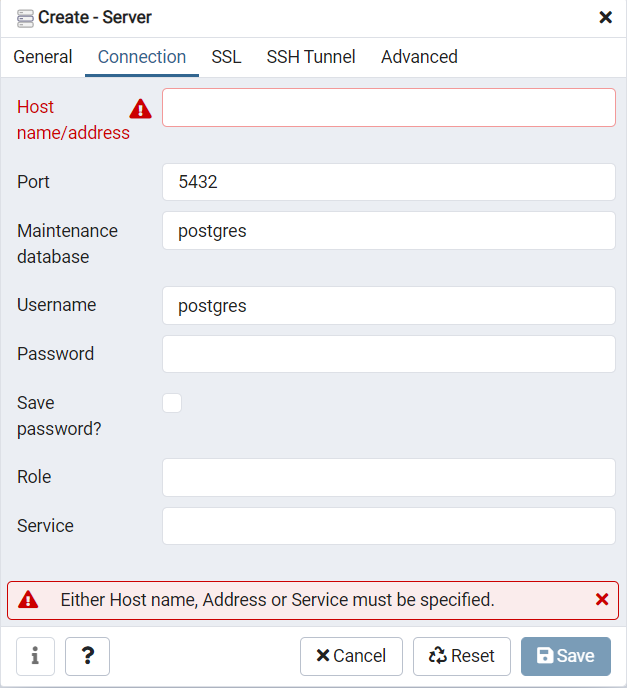

2.2 Creating a Database

Open the Databases tree item and have a look at the available databases. The postgres database is the user database for the default postgres user and is not too interesting to us.
Right-click on the Databases item and select New Database.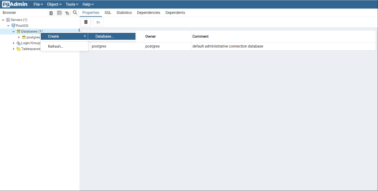
Fill in the Create Database form as shown below and click OK.

Name nyc

Owner postgres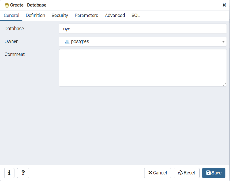
Select the new nyc database and open it up to display the tree of objects. You'll see the public schema.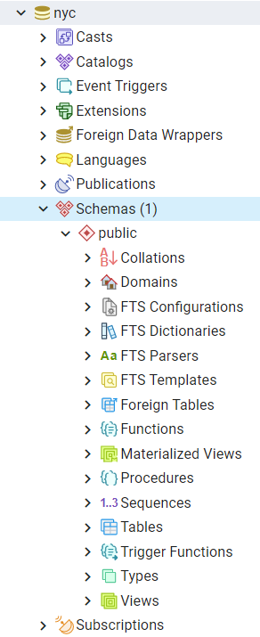
Click on the SQL query button indicated below (or go to Tools > Query Tool).
Enter the following query into the query text field to load the PostGIS spatial extension:
```
CREATE EXTENSION postgis;
```
Click the Play button in the toolbar (or press F5) to "Execute the query."
Now confirm that PostGIS is installed by running a PostGIS function:
```
SELECT postgis_full_version();
```

You have successfully created a PostGIS spatial database!!

2.3 Function List

PostGIS_Full_Version: Reports full PostGIS version and build configuration info.

3 Loading spatial data

Supported by a wide variety of libraries and applications, PostGIS provides many options for loading data.

We will first load our working data from a database backup file, then review some standard ways of loading different GIS data formats using common tools.

3.1 Loading the Backup File

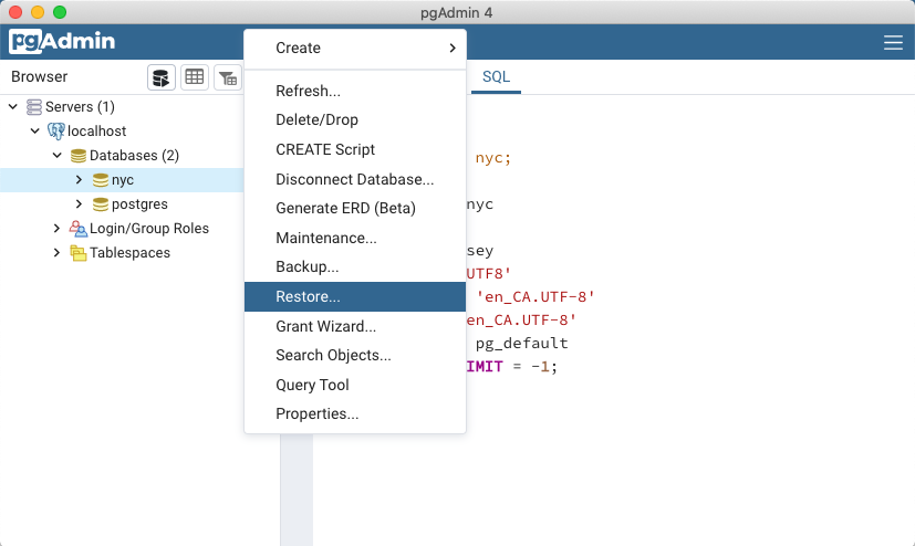
In the PgAdmin browser, right-click on the nyc database icon, and then select the Restore... option.

{.inline, .border .inline, .border}
Browse to the location of your workshop data data directory (available in the workshop data bundle), and select the nyc_data.backup file.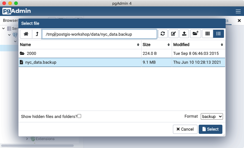

{.inline, .border .inline, .border}
Click on the Restore options tab, scroll down to the Do not save section and toggle Owner to Yes.

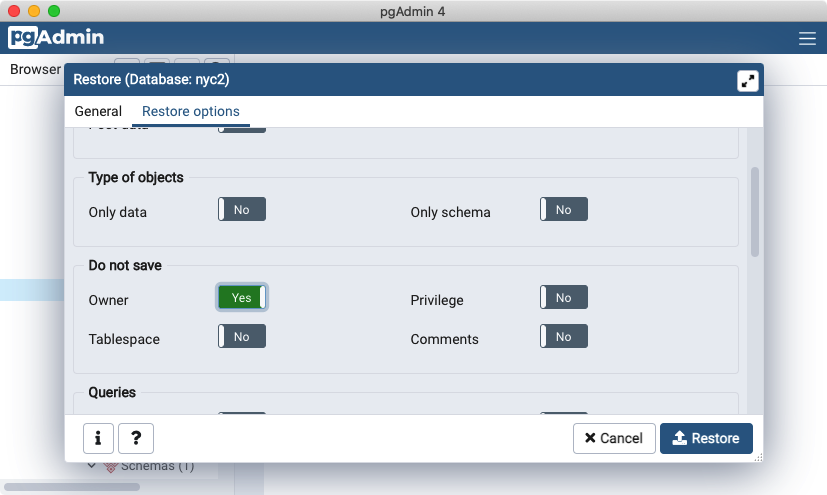{.inline, .border .inline, .border}
Click the Restore button. The database restore should run to completion without errors.

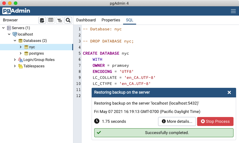{.inline, .border .inline, .border}
After the load is complete, right click the nyc database, and select the Refresh option to update the client information about what tables exist in the database.

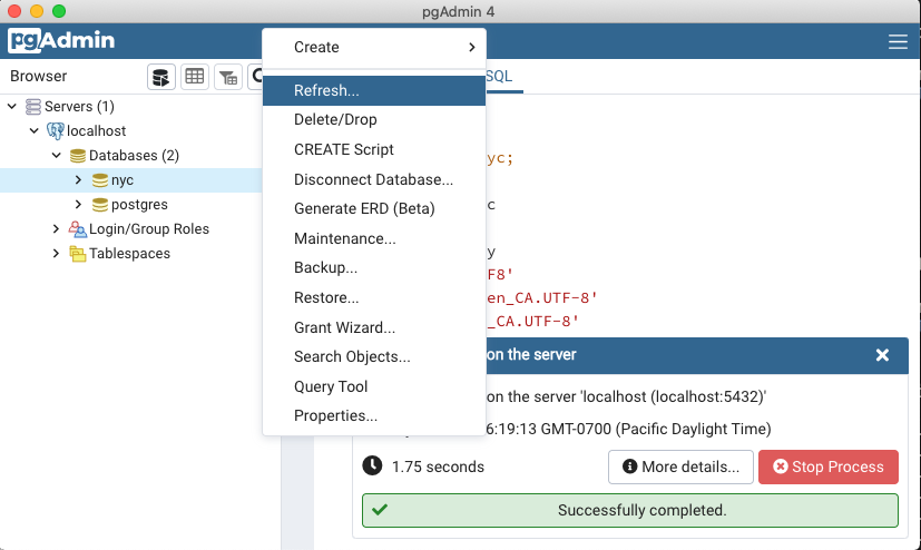{.inline, .border .inline, .border}

Note

If you want to practice loading data from the native spatial formats, instead of using the PostgreSQL db backup files just covered, the next couple of sections will guide you thru loading using various command-line tools and QGIS DbManager. Note you can skip these sections, if you have already loaded the data with pgAdmin.

3.2 Shapefiles? What's that?

You may be asking yourself -- "What's this shapefile thing?" A "shapefile" commonly refers to a collection of files with .shp, .shx, .dbf, and other extensions on a common prefix name (e.g., nyc_census_blocks). The actual shapefile relates specifically to files with the .shp extension. However, the .shp file alone is incomplete for distribution without the required supporting files.

Mandatory files:

.shp—shape format; the feature geometry itself
.shx—shape index format; a positional index of the feature geometry
.dbf—attribute format; columnar attributes for each shape, in dBase III

Optional files include:

.prj—projection format; the coordinate system and projection information, a plain text file describing the projection using well-known text format

The shp2pgsql utility makes shape data usable in PostGIS by converting it from binary data into a series of SQL commands that are then run in the database to load the data.

3.3 Loading with shp2pgsql

The shp2pgsql converts Shape files into SQL. It is a conversion utility that is part of the PostGIS code base and ships with PostGIS packages. If you installed PostgreSQL locally on your computer, you may find that shp2pgsql has been installed along with it, and it is available in the executable directory of your installation.

Unlike ogr2ogr, shp2pgsql does not connect directly to the destination database, it just emits the SQL equivalent to the input shape file. It is up to the user to pass the SQL to the database, either with a "pipe" or by saving the SQL to file and then loading it.

Here is an example invocation, loading the same data as before:

export PGPASSWORD=mydatabasepassword

shp2pgsql \
  -D \
  -I \
  -s 26918 \
  nyc_census_blocks_2000.shp \
  nyc_census_blocks_2000 \
  | psql dbname=nyc user=postgres host=localhost

Here is a line-by-line explanation of the command.

shp2pgsql \

The executable program! It reads the source data file, and emits SQL which can be directed to a file or piped to psql to load directly into the database.

-D \

The D flag tells the program to generate "dump format" which is much faster to load than the default "insert format".

-I \

The I flag tells the program to create a spatial index on the table after loading is complete.

-s 26918 \

The s flag tells the program what the "spatial reference identifier (SRID)" of the data is. The source data for this workshop is all in "UTM 18", for which the SRID is 26918 (see below).

nyc_census_blocks_2000.shp \

The source shape file to read.

nyc_census_blocks_2000 \

The table name to use when creating the destination table.

| psql dbname=nyc user=postgres host=localhost

The utility program is generating a stream of SQL. The "|" operator takes that stream and uses it as input to the psql database terminal program. The arguments to psql are just the connection string for the destination database.

3.4 SRID 26918? What's with that?

Most of the import process is self-explanatory, but even experienced GIS professionals can trip over an SRID.

An "SRID" stands for "Spatial Reference IDentifier." It defines all the parameters of our data's geographic coordinate system and projection. An SRID is convenient because it packs all the information about a map projection (which can be quite complex) into a single number.

You can see the definition of our workshop map projection by looking it up either in an online database,

https://epsg.io/26918

or directly inside PostGIS with a query to the spatial_ref_sys table.

SELECT srtext FROM spatial_ref_sys WHERE srid = 26918;

Note

The PostGIS spatial_ref_sys table is an OGC-standard table that defines all the spatial reference systems known to the database. The data shipped with PostGIS, lists over 3000 known spatial reference systems and details needed to transform/re-project between them.

In both cases, you see a textual representation of the 26918 spatial reference system (pretty-printed here for clarity):

PROJCS["NAD83 / UTM zone 18N",
  GEOGCS["NAD83",
    DATUM["North_American_Datum_1983",
      SPHEROID["GRS 1980",6378137,298.257222101,AUTHORITY["EPSG","7019"]],
      AUTHORITY["EPSG","6269"]],
    PRIMEM["Greenwich",0,AUTHORITY["EPSG","8901"]],
    UNIT["degree",0.01745329251994328,AUTHORITY["EPSG","9122"]],
    AUTHORITY["EPSG","4269"]],
  UNIT["metre",1,AUTHORITY["EPSG","9001"]],
  PROJECTION["Transverse_Mercator"],
  PARAMETER["latitude_of_origin",0],
  PARAMETER["central_meridian",-75],
  PARAMETER["scale_factor",0.9996],
  PARAMETER["false_easting",500000],
  PARAMETER["false_northing",0],
  AUTHORITY["EPSG","26918"],
  AXIS["Easting",EAST],
  AXIS["Northing",NORTH]]

If you open up the nyc_neighborhoods.prj file from the data directory, you'll see the same projection definition.

Data you receive from local agencies—such as New York City—will usually be in a local projection noted by "state plane" or "UTM". Our projection is "Universal Transverse Mercator (UTM) Zone 18 North" or EPSG:26918.

3.5 Things to Try: View data using QGIS

QGIS, is a desktop GIS viewer/editor for quickly looking at data. You can view a number of data formats including flat shapefiles and a PostGIS database. Its graphical interface allows for easy exploration of your data, as well as simple testing and fast styling.

Try using this software to connect your PostGIS database. The application can be downloaded from https://qgis.org

You'll first want to create a connection to a PostGIS database using menu Layer->Add Layer->PostGIS Layers->New and then filling in the prompts. Once you have a connection, you can add Layers by clicking connect and selecting a table to display.

3.6 Loading data using QGIS DbManager

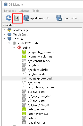
QGIS comes with a tool called DbManager that allows you to connect to various different kinds of databases, including a PostGIS enabled one. After you have a PostGIS Database connection configured, go to Database->DbManager and expand to your database as shown below:

{.inline, .border .inline, .border}

From there you can use the Import Layer/File menu option to load numerous different spatial formats. In addition to being able to load data from many spatial formats and export data to many formats, you can also add ad-hoc queries to the canvas or define views in your database, using the highlighted wrench icon.

This section is based on the PostGIS Intro Workshop, sections 3, 4, 5,and 7

Name	`nyc`
Owner	`postgres`